Answering visual queries with attention
One of the most common building blocks of neural networks is attention. Attention mechanisms, first introduced in a few years ago in the context of neural machine translation1, help a model focus on what’s important for the task at hand. A great overview is this blog post, that mentions a number of different flavors and applications of attention.
Consider a setting where we have an image $x$ that contains a number of symbols, with different colors, sampled from a finite alphabet $\Gamma$. Let $\gamma$ be a query image, that contains the representation of a symbol from $\Gamma$. Then, given the pair $(x,\gamma)$, what is the color (in the image $x$) of the symbol represented in the query image $\gamma$? We can use some sort of visual attention to answer the question.
Colored MNIST
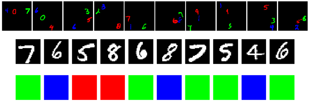
Consider the MNIST dataset, that contains 10 “symbols” (the 0 to 9 digits). We can define a new ColoredMNIST dataset, as a (more or less) infinite stream where each sample contains:
- a query B&W image $\gamma$, randomly extracted from MNIST;
- an input RGB image $x$, with 3 differently colored symbols from MNIST;
- the target color (that is, the color of the queried symbol within the input image). For sake of simplicity, we use only the 3 primary colors, RGB, so that $y \in [0,1,2]$.
Here’s a batch of 10 generated examples:
The idea is to learn a model that, at inference time, can focus its attention on different locations of the input image based on the content of the query. Here’s a simple architecture:
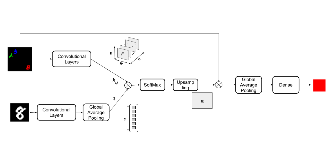
The lower branch of the network encodes the query image $\gamma$ into a vector $q \in \mathbb{R}^c$. The upper branch of the network encodes the input image $x \in \mathbb{R}^{3 \times h\times w}$ into a feature map $K\in \mathbb{R}^{c \times h’\times w’}$, that can be seen as a set of feature vectors $k_{ij}\in \mathbb{R}^c$ for each position $(i,j)$. Then, for each location $(i,j)$, we compute a similarity score between the local features $k_{ij}$ and the query $q$:
\[score(q, k_{ij}) = \frac{q^Tk_{ij}}{\sqrt{n}}\]The score measures if the model should focus on the position $(i,j)$, given the input query $q$, using a simple scaled dot-product attention2. The final attention mask is obtained applying a (spatial) softmax on the obtained scores.
\[\alpha_{ij} = \frac{\exp(score(q, k_{ij}))}{\sum_{i'j'} \exp(score(q, k_{i'j'}))}\]The resulting mask $\alpha \in R^{h’\times w’}$ is upsampled to the size of the input image, and used to attend to the part of the input image that better matches the query.
At this point, if the attention mechanism has focused on the correct symbol, and discarded the rest of the image, taking a Global Average Pooling over the masked image should yield a 3-dimensional vector whose argmax is exactly the prediction we want.
(Here's the pytorch code to define the model.)
class ColorNetImage(nn.Module):
    """
    1. Extract set of spatial features from input image
    2. Extract set of features from query image
    3. Use those features to query the features from the input image in space
    4. Use attention mask to extract a glimpse of the input image
    5. Classify it with a final global average pooling + dense
    """
    def __init__(self, debug=False):
        super().__init__()
        self.conv_features = nn.Sequential(
                       nn.Conv2d(3, 8, 5, stride=2, padding=2),
                       nn.BatchNorm2d(8),
                       nn.ReLU(),
                       nn.Conv2d(8, 16, 3, stride=2, padding=1),
                       nn.BatchNorm2d(16),
                       nn.ReLU(),
                       nn.Conv2d(16, 32, 3, stride=2, padding=1),
                       nn.BatchNorm2d(32),
                       nn.ReLU()
        )
        self.query_features = nn.Sequential(
                       nn.Conv2d(1, 8, 5, stride=2, padding=2),
                       nn.BatchNorm2d(8),
                       nn.ReLU(),
                       nn.Conv2d(8, 16, 3, stride=2, padding=1),
                       nn.BatchNorm2d(16),
                       nn.ReLU(),
                       nn.Conv2d(16, 32, 3, stride=2, padding=1),
                       nn.BatchNorm2d(32),
                       nn.ReLU()
                    )
        self.fc = nn.Linear(3, 3)
        self.fc.weight.data = 60*torch.eye(3) - 10

    def forward(self, x, debug=False):
        image, query = x["image"], x["query"]
        N = image.size(0)

        K = self.conv_features(image)
        Q = F.adaptive_avg_pool2d(self.query_features(query), 1).view(N,-1)

        # Dot-product attention. Compute score(K(i,j),Q) for each (i,j)
        score = torch.einsum('bcij,bc->bij', K, Q)/np.sqrt(K.size(1))
        alpha = F.softmax(score.view(N, -1), dim=1).view_as(score).unsqueeze(1)
        alpha_upsampled = F.interpolate(alpha, size=(image.size(2), image.size(3))).squeeze(1)

        # Then use alpha to mask the input image
        masked = torch.einsum('bcij,bij->bcij', image, alpha_upsampled)

        # Global average pooling + a tiny dense to help with scaling
        out = self.fc(F.adaptive_avg_pool2d(masked, 1).view(N, -1))

        if debug:
            return out, score, alpha_upsampled
        return out
This (small) model has 12668 trainable parameters. I set an epoch to contain 10000 samples (an arbitrary number, since the training set is effectively infinite). At the end of each epoch the performance is validated on a held-out set of 1000 examples. I used Adam with learning rate 0.001, and a batch size of 128. Each epoch takes roughly 7/8 seconds in Google Colab (with an NVidia T4 – by the way, Colab is awesome for this kind of quick experiments). After a hundred training epochs (around 10 minutes), the model reaches more than 90% accuracy on the validation set, and you can easily get up to 95% if you keep training. Still far from the 98%+ accuracy one easily gets on MNIST with a similarly sized CNN, showing there’s significant room for improvement here.
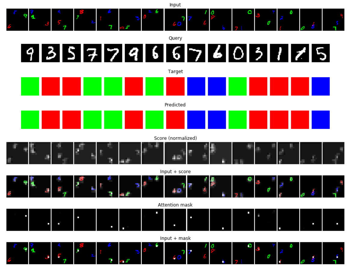
This is an example of the predictions of the best model on a batch of randomly generated data:
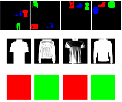
Similar results, with slightly worse accuracy (~85%), can be obtained on FashionMNIST.
Things that worked
- Good initialization and input normalization.
- To avoid any risk of overfitting, the training samples must be generated randomly and non-deterministically for each batch and epoch; while the (random) validation set must be generated in a deterministic way, to obtain comparable results.
- In principle, since the task is simply to predict one of the 3 primary colors, applying a Global Pooling on the masked image would be enough. However, since only a small portion of the mask image will be non-zero, the spatial average of the 3 channels will be very similar (close to 0) and the output of the final softmax will be almost uniform. It is super-helpful to add a scaling with a linear layer, initialized with a diagonal-heavy matrix.
- Padding is helpful to ensure that the size of $K$ is a multiple of the input image. This way, after the upsampling, the attention mask maps precisely to the input image. Without padding, small localization errors are introduced, bringing down the overall accuracy a little bit.
- Unsurprisingly, adding batch normalization helps.
What didn’t work
- Using attention to attend to the feature map $K$ itself, rather than the raw input image $x$. It led to much slower convergence and inferior results; the attention mask was also much less interpretable – it didn’t focus on the correct area of the image.
- An (extremely) silly, no-learning baseline: compute the spatial convolution between the query image and the input image, and take the argmax (the silliest kind of pattern matching). It didn’t work at all (only a bit better than random guessing).
Things one could have tried – but I didn’t, for lack of time
- Pre-training the encoders on MNIST.
- Fiddling with the architecture – the training is a bit too slow, something might be off.
- Fiddling with hyperparameters and/or learning rate schedules. The loss goes down pretty quickly at the beginning; when the training seems to plateau, reducing the learning rate could help.
A notebook with all the code needed to define the dataset and train the model can be found here. It can also be easily run on CPU (an epoch takes roughly 20 seconds on my laptop).