Some thoughts on MINLP problems
Lately, I’ve had to deal with mixed-integer nonlinear programming (MINLP) models. I’ll share a couple of considerations – and show one weird trick to reduce your optimization time by 99.96% adding just a single, simple cut! You can thank me later.
I’ve experimented with some global solvers (SCIP, BARON, Couenne) on a nonconvex MINLP problem. Bringing together two inherently difficult aspects as nonconvexity and integrality sure is an arduous task. I would say that MINLP solvers (and theory, and algorithms?) are less mature than their linear counterparts, although it is a very active field of research.
What I’ve seen is that even small details in the formulation are crucial (no big surprise, I guess):
- Scaling – Scaling is important. At one point I had an instance whose variables could assume values over 10^6. I thought that wasn’t ideal, but hopefully it wouldn’t cause too many problems. It did. Those variables were squared in a constraint, and the solvers would either a) fail b) issue some cryptic warning c) say nothing, and return a plainly wrong result (actually, an infeasible solution). Manual scaling was necessary.
- Bounds – If you don’t provide any bounds, you’d better be a really patient guy. Even what look like trivial bounds are essential.
- Cutting planes – This is what inspired me to write this post. MINLP solvers apply manipulations and reformulations of the nonlinear expressions. However, my feeling is that, in doing so, some important structure of the problem might be missed. Sometimes even the simplest valid inequalities are helpful in cutting down the solving time.
As an example for point 3, I solve a small instance of a nonlinear multi-item production planning problem with 168 variables (24 binary) and 240 constraints. I’ll describe the model later.
| Solver | Time (s) | Nodes | Gap% |
|---|---|---|---|
| SCIP 3.1 | 49.8 | 94882 | 0.00 |
| BARON 10.2 | 1563.4 | 156520 | 1.00 |
This small problem seems already to be nontrivial for state-of-the-art global solvers (to be fair, that is not the most recent version of Baron).
Is it really hard already, or are the solvers missing something? Can we help them in any way?
Adding a single, very simple cutting plane (details in the next paragraph, pictures included), you get these results:
| Solver | Time (s) | Nodes | Gap% |
|---|---|---|---|
| SCIP 3.1 | 0.02 | 1 | 0.00 |
| BARON 10.2 | 0.18 | 1 | 0.00 |
Now both solvers breeze through it, solving the problem in the root node. It is pretty remarkable how effective the cutting plane was.
This valid inequality doesn’t always make such an impact – hey, it’s just one cutting plane, what do you expect? But in quite a few of my instances, it seems to be very useful. Why is that the case?
#The gory details
Here is a basic formulation of the nonlinear production planning problem mentioned above. Simple AMPL and GAMS implementations can be found here.
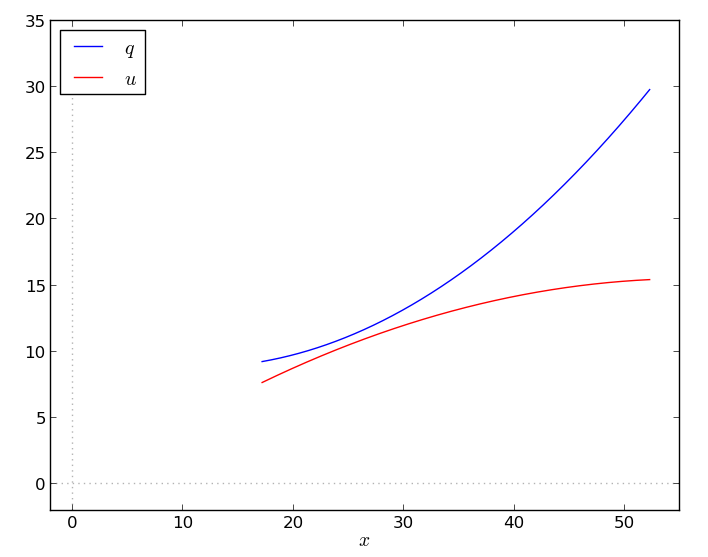
\[\begin{align} \min\quad & \sum_{t\in T}\left(b_tz_t + c_t x_t + h_t q^{+}_t - p_tq^{-}_t\right) & \\ s.t.\quad & q_t + q^{+}_t - q^{-}_t = d^{q}_t \qquad& \tag{1} \forall t \in T \\ & u_t + s_t \ge d^{u}_t + s_{t+1} \qquad&\tag{2}\\ & z_tX^{min} \le x_t \le z_tX^{max}\qquad&\tag{3}\\ & q_t \le z_tf(x_t) \qquad&\tag{4} \\ & u_t \le z_tg(x_t) \qquad&\tag{5} \\ & q_t, u_t, q^{+}_t, q^{-}_t \ge 0 \qquad&\\ & 0 \le s_t \le S \qquad&\\ & z_t \in\{0,1\} \qquad& \end{align}\]We have one production plant that, given an input quantity \(x_t\), provides two commodities \(q_t\) and \(u_t\). We want to decide when and how much to produce in order to satisfy the demands \(d^q_t\) and \(d^u_t\) in each hour, minimizing the total costs.
The production is nonlinear and is a function of the variable \(x_t\) via \(f(\cdot)\) and \(g(\cdot)\), if the plant is on (4–5). Constraints (3) impose technical bounds on the input quantity \(x_t\) (i.e., minimum and maximum lot size). The plant produces the commodities simultaneously, but according to different “performance curves”.
Constraints (1) and (2) are simple balance constraints. This is not extremely important here, but the items we produce are managed differently. Commodity \(q_t\) can be sold, if in excess, and bought (back-ordered), if the production is not sufficient (1). Commodity \(u_t\) can be stocked for the following time slot. Storing is free, but we have an upper bound \(S\) on the quantity in stock (2). Quantity in excess can be discarded with no additional costs.
If \(f\) and \(g\) are both concave, this problem is (or can be reformulated as) a convex MINLP. However, it may well be the case that \(f\) and \(g\) are not concave. Assume that, for commodity \(u_t\), the plant is more efficient at lower loads, “saturating” as \(x\) grows (\(g\) is concave); while the production of \(q_t\) increases its efficiency as \(x_t\) grows (\(f\) is convex). This leads to a nasty nonconvex MINLP.
If you simply approximate the nonlinear functions with piecewise linear ones (and use a big-M term) you can solve the resulting MILP with your favorite solver in a matter of seconds (or less), even for quite large-size instances.
Going back to the original MINLP, let’s plot the feasible region defined by the constraint \(q_t \le z_tf(x_t)\):
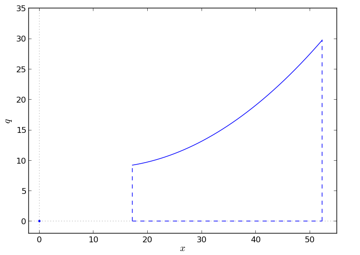
Points in the optimal solution are going to lie either in the origin (\(z_t\) is 0, so production is off) or on the graph of \(f\) in the feasible domain \([X^{min},X^{max}]\).
The simplest (upper) convex hull approximation you can take is the line connecting the extreme point \((X^{max}, f(X^{max}))\) and the origin (0,0) – assuming, as it is the case, that \((X^{min}, f(X^{min}))\) lies under the line.
[Otherwise, you can have a cutting plane just taking the line through \((X^{min}, f(X^{min}))\) and \((X^{max}, f(X^{max}))\). I think you can call that a secant approximation of \(f\).]
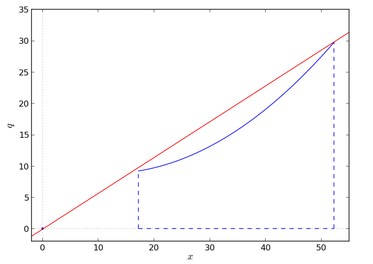
And this is the glorious cutting plane that achieves the remarkable speed-up reported above.
Note that the cut is so effective probably because the curve, in that instance, is actually quite close to being linear. But, are solvers really missing that cutting plane? It looks to me that would be one of the easiest thing you could come up with.
Is perhaps my initial formulation not good for the solvers – maybe it’s not what they expect at all? I’ve tried quite a few equivalent formulations (e.g., replacing the product in (4–5) with big-M terms, or projecting out variables \(x_t\)), but I’ve seen no big difference. Still, I’m not really used to working with MINLP solvers, so that just might be the case.
Anyway, I sure wish it happened more often that such an easy trick could be this effective.