Google Hash Code 2017: streaming videos
Google Hash Code is an algorithmic competition organized by Google, open to European and African participants, in teams of no more than 5 people. The way it works is simple: you have 4 hours, a problem statement, 4 datasets, and you need to submit a solution for each dataset so that your total score – i.e., the sum of the individual scores – is maximized. The problems so far have always been combinatorial optimization ones. Last year’s competition (2016) was about optimizing the routes of delivery drones. This year, the competition was about optimizing the assignment of videos to cache servers in a distribution network that connects a main data center to a number of endpoints.
I really don’t have the time for these things right now… but I’m a sucker for them!
The problem
This year, the problem was related to caching in distributed video infrastructures – such as YouTube. As more and more people watch online videos (and as the size of these videos increases), the video-serving infrastructure must be optimized to handle requests reliably and quickly. This typically involves putting in place cache servers, which store copies of popular videos. When a user request for a particular video arrives, it can be handled by a cache server close to the user, rather than by a remote data center thousands of kilometers away. But how should Google decide which videos to put in which cache servers?
Given a description of cache servers, network endpoints and videos, along with predicted requests for individual videos, the task is to decide which videos to put in which cache server in order to minimize the average waiting time for all requests. The picture below represents the video serving network.
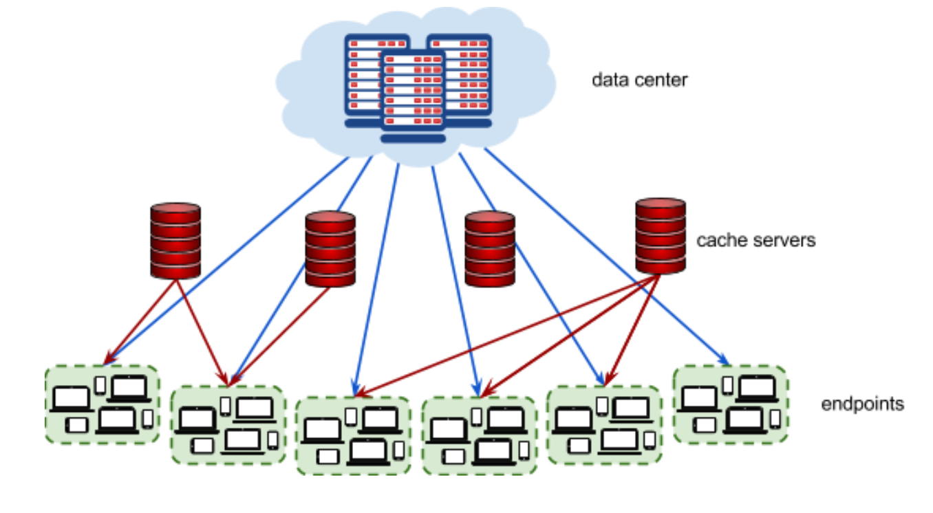
Each video \(v\in V\) has a size \(S_v\) given in megabytes (MB). The data center stores all videos. Additionally, each video can also be put in 0, 1, or more cache servers. Each cache server \(c \in C\) has a maximum capacity \(X\), given in megabytes.
Each endpoint \(e \in E\) represents a group of users connecting to the Internet in the same geographical area (for example, a neighborhood in a city). Every endpoint is connected to the data center.
Each endpoint is characterized by the latency \(L_{d,e}\) of its connection to the data center (how long it takes to serve a video from the data center to a user in this endpoint), and by the latencies \(L_{c,e}\) to each cache server (how long it takes to serve a video stored in the given cache server to a user in this endpoint). Finally, the predicted requests \(n_{e,v}\) provide data on how many times a particular video \(v\) is requested from a particular endpoint \(e\).
The aim is to minimize the average delay of the requests; for each request \((v,e)\), the delay is computed as the minimum latency between the endpoint \(e\) and any source that contains the video, i.e., the data center or any cache server where it’s stored.
The PDF with the full description can be found here, along with more information on the format of the data files. The problem can be summarized in a succint way like this:
\[\begin{align} \min & \frac{\sum_{e \in E, v \in V} n_{e,v} \min \left\{ L_{d,e}, \min_{c \in C} \{L_{c,e} | x_{v,c} = 1\} \right\}}{\sum_{e \in E, v \in V} n_{e,v}}\\ %\min & \sum_{r \in R} n_r \min \left\{ L_{d,e_r}, L_{c,e_r} \cdot x_{v_r,c}} \right\}\\ &\sum_{v \in V}S_v \cdot x_{v,c} \leq X \qquad \forall c\in C\\ & x_{v,c} \in \{0,1\} \qquad \forall v \in V, c\in C \end{align}\]where the only decision variables are the binary variables \(x_{v,c}\) that assign a video \(v\) to a cache server \(c\), and the only constraint is the capacity of the cache servers that must not be exceeded. However, the objective function is quite complicated, and makes the problem challenging.
The four instances that were given are summarized in the next table.
| name | num.videos | num. cache servers | num. endpoints | distinct requests |
|---|---|---|---|---|
me_at_the_zoo |
100 | 10 | 10 | 81 |
trending_today |
10000 | 100 | 100 | 95180 |
video_worth_spreading |
10000 | 100 | 100 | 40317 |
kittens |
10000 | 500 | 1000 | 197978 |
How you want to solve it
During the very short 4 hours (actually 3h and 45m), given the quite involved problem description, the thing you probably want to do is quickly write down a sensible heuristic, and then start improving upon your solutions, with some kind of local search, until the time’s up.
This is what we tried to do. Coordinating in such a short time is quite a challenge – if you and your teammates are not on the same page, you end up wasting a whole lot of precious time. And that totally happened to us, so yeah, we didn’t end up in the top 20 teams that had access to the final round in Paris..
In hindsight, I also believe that the time of a team member might actually be well spent in trying to look at the data, and see if there is something particular pattern you can exploit: in one instance, all the server-endpoints latencies were identical. I didn’t even realize that until the day after, when I looked at the data on my own.
Integer programming? Why not!
Something else that one could try (and indeed, you should always give it a try.. it might just work!) was, of course, integer programming. The objective function is nonconvex, fine. But it can be easily linearized with the help of a bunch extra binary variables and constraints.
\[\begin{align} \min & \sum_{e \in E, v \in V} n_{e,v} \eta_{e,v} \\ s.t.&\sum_{v \in V}S_v \cdot x_{v,c} \leq X & \forall c\in C \tag{1}\\ & \eta_{e,v} \geq L_{c,e} \sigma_{e,c,v} & \forall e \in E, c \in C, v \in V\tag{2}\\ & \eta_{e,v} \geq L_{d,e}\left(1 - \sum_{c \in C}\sigma_{e,c,v}\right) & \forall e \in E, v \in V\tag{3}\\ & \sigma_{e,c,v} \leq x_{v,c} &\forall e \in E, c \in C, v \in V \tag{4}\\ & x_{v,c} \in \{0,1\} & \forall v \in V, c\in C\\ & \eta_{e,v} \ge 0 & \forall e \in E, v \in V\\ & \sigma_{e,c,v} \in \{0,1\} & \forall e \in E, v \in V, c \in C\\ %& \zeta_{e,v} \in \{0,1\} & \forall e \in E, v \in V% \end{align}\]Each binary variable \(\sigma_{e,c,v}\) indicates whether the cache server \(c\) is the one that will serve the video \(v\) to the endpoint \(e\), that is, it is the server with minimum latency to the endpoint \(e\) among all those that contain the video \(v\). If none of them is selected, it means that we have chosen to serve the video \(v\) to \(e\) straight from the data center.
The value of the variable \(\eta_{e,v}\) in an optimal solution, will be equivalent to the minimum latency from \(v\) to \(e\) (either from the closest cache server that contains \(v\), or the data center).
The logic is simple, standard integer programming tricks: Constraint (3) ensures that the latency for \((e,v)\) will equal to the latency from the cache server we have selected to serve that video. This works due to the fact that we are minimizing, and in an optimal solution, only the server with minimum latency will be selected. (If that’s not the case, it’s easy to see that the solution cannot be optimal.)
Constraints (4) ensure that, if no cache server is actually selected for a request \((e,v)\), then the latency will be equal to the latency from the data center. If a cache server is selected, this constraint won’t be active.
Finally, the auxiliary variables must be linked to the assignment variables \(x\): a cache server can be chosen to serve a request \((e,v)\) only if the video \(v\) has actually been assigned to it (\(x_{v,c} = 1\)) – and this is ensured by Constraint (5).
Even if it’s pretty easy to write and understand, this 3-index formulation can grow quickly in size: indeed, for the largest instances in the dataset, the number of variables and constraints is huge. One could probably try to find a more compact one, or a stronger one. But let’s give it a spin anyway.
This formulation can be translated into your favorite modeling language (I’ll pick JuMP).
In the following code, V[e] is the set of videos such that \(n_{e,v} > 0\), and C[e] is the set of cache servers
such that \(L_{c,e} < L_{d,e}\). (Yes, this is working code, with all the cool unicode symbols.)
    m = Model(solver=GurobiSolver(Threads=1))
    #m = Model(solver=CplexSolver())

    # Assignment variables
    @variable(m, x[V,C], Bin)

    # Auxiliary variables: minimum delay for video v from endpoint e
    @variable(m, η[e in E, v in V[e]] ≥ 0)

    # Auxiliary variables: σ[e,c,v] = 1 if the cache server c has been chosen to serve video v
    # for endpoint e, i.e., it has minimum delay for video v from endpoint e
    @variable(m, σ[e in E, c in C[e], v in V[e]], Bin)

    # Objective function
    @objective(m, Min, sum(num_req[e][v]*η[e,v] for e in E, v in V[e]) ) )

    # Capacity constraint
    @constraint(m, capacity[c in C], ∑(S[v]*x[v,c] for v ∈ V) ≤ X)

    # If v is not in the cache server c, then c cannot be selected
    # for the request (e,v)
    for e ∈ E, c ∈ C[e], v ∈ V[e]
        @constraint(m, σ[e,c,v] ≤ x[v,c])
    end

    # Ensure η takes the correct value in an optimal solution
    for e ∈ E, c ∈ C[e], v ∈ V[e]
        # The latency for a request is either the latency from the selected cache server..
        @constraint(m, η[e,v] ≥ L[e][c] * σ[e,c,v])
    end
    for e ∈ E, v ∈ V[e]
        # .. or the latency from the data center.
        @constraint(m, η[e,v] ≥ Ld[e] * (1 - ∑(σ[e,c,v] for c in C[e]) )
    end
With this model, the smallest instance, me_at_the_zoo, is solved in a fraction of a second with any state-of-the-art integer programming solver. No need to take out your big heuristic guns just yet:
Optimize a model with 694 rows, 1423 columns and 2548 nonzeros
...

Nodes    |    Current Node    |     Objective Bounds      |     Work
 Expl Unexpl |  Obj  Depth IntInf | Incumbent    BestBd   Gap | It/Node Time

     0     0 4512675.38    0   43 3.2469e+07 4512675.38  86.1%     -    0s
H    0     0                    5616356.0000 4512675.38  19.7%     -    0s

...

Cutting planes:
  Gomory: 5
  Cover: 36
  Clique: 2
  MIR: 26
  GUB cover: 1
  Zero half: 2

Explored 333 nodes (3630 simplex iterations) in 0.31 seconds
Thread count was 1 (of 8 available processors)

Optimal solution found (tolerance 1.00e-04)
Best objective 4.930602000000e+06, best bound 4.930602000000e+06, gap 0.0%
Optimal savings as per the objective function: 516557.0 ms
and that’s it, half a second to the global optimum. Of course, it’s a reasonably small problem for current MIP solvers – although combinatorial problems can be extremely hard even with tiny instances.
The two medium ones.. they are already rather big. The number of variables and constraints in the linearized formulation
is in the millions.
But, as I mentioned, one of them, trending_videos, actually had all the
cache servers latencies to any end point with the same value, that is, \(L_{c,e} = L_c ~\forall e \in E, c \in C\).
and the same for the data center latencies, i.e., \(L_{d,e} = L_d ~\forall e \in E\).
You still need to decide where to allocate the videos, but the objective function is much easier to linearize, since you only need to take care of considering the case where you have assigned the video to at least a cache server, or you haven’t, but you don’t actually have to do the book-keeping to check which server is the closest.
So a simpler linearized formulation would be:
\[\begin{align} \min & \sum_{e \in E, v \in V} n_{e,v} \eta_{e,v} \\ s.t.&\sum_{v \in V}S_v \cdot x_{v,c} \leq X & \forall c\in C \\ & \zeta_{e,v} + \sum_{c \in C}x_{v,c} = 1 & \forall e \in E, v \in V\\ & \eta_{e,v} \geq L_{d} \zeta_{e,v} + L_c ( 1 - \zeta_{e,v} ) & \forall e \in E, v \in V\\ & x_{v,c} \in \{0,1\} & \forall v \in V, c\in C\\ & \eta_{e,v} \ge 0 & \forall e \in E, v \in V\\ & \zeta_{e,v} \in \{0,1\} & \forall e \in E, v \in V% \end{align}\]where \(\zeta_{e,v}\) indicates whether the data center has been selected to serve the video \(v\) to the endpoint \(e\), that becomes:
for e ∈ E, v ∈ V[e]
    # For each video v requested from e, either it is assigned to a cache server,
    # or it is served from the data center.
    @constraint(m, ζ[e,v] + ∑(x[v,c] for c in keys(L[e])) == 1)

    # If v is served from the data center, the delay is Ld
    # otherwise it is Lc
    @constraint(m, η[e,v] ≥ Ld * ζ[e,v] + Lc * (1 - ζ[e,v]) )
end
This is still a problem with more than 1 million variables, but modern MIP codes will solve it in a few minutes.
For the third instance, video_worth_spreading, you need to use the full formulation. It’s big enough to be challenging to solve to global optimality, but if you
throw in a heuristic solution as a warm start, the solver will gladly improve it.
Now, for the largest one, kittens: yup, I reckon it seems a bit too much. At the very bare minimum,
the problem has 5 millions assignment variables, not even counting the extra linearization variables and constraints..
where those \(O(|V||E||C|)\) make your model explode in size.
But I’m pretty sure you could at least build a successful heuristic around the integer programming formulation – you might want to prune the state space by discarding non-promising variables, or maybe write an aggregate formulation to reduce the number of variables. Not to mention that one might want to try some more dynamic technique (cutting planes, or a decomposition approach).
The full, ugly code with this formulation and some utility functions, along with the even uglier code we wrote during the competition, can be found in this repo.