Playing with probabilistic data structures
When dealing with streams of data, we might sometimes need to count or compute some statistics of the stream. This may bring about practical issues – typically, efficiency and/or space concerns. In some cases, probabilistic data structures come in handy.
These structures are something I had never studied during the university days - though hash tables may be seen as belonging to this class. They are simple and very clever ideas, but they’re best suited for very specific applications.
In this github repo here I implemented and tested two such structures: the Count-Min Sketch and the Bloom Filter.
Count-Min Sketch
Count-Min Sketch, introduced in [1], is a structure used to keep an approximate count of each distinct value seen in a data stream. The idea is to encode the values seen in the stream in an aggregated way, with obvious gain in space, at the cost of collisions. The idea is super simple: assuming we expect roughly \(N\) distinct values, keep a \(d \times w\) table \(X\), with \(w \ll N\). Each row is associated to a hash function $h_i: \mathbb{N} \to [0,w]$. When a new value \(v\) comes in, for each row i, we add 1 to the $h_i(v)$-th cell. This way, in a given row, collisions will occur for distinct values that are mapped by \(h_i\) to the same cell. However, having \(d\) rows, will reduce the chance of collisions. To query the count of a value \(v\), then, it is enough to take the minimum of the count of that value in each row, i.e., $\min_{i \in D}X_{i,h_i(v)}$. A minimal implementation is the following, where I implemented simple hash functions as suggested in [2]:
import numpy as np

class CountMinSketch:
    def __init__(self, d: int, w: int):
        self.X = np.zeros((self.d, self.w), dtype=int)
        self.hash = Hash(self.d, self.w)

    def update(self, x: int, v: int=1):
        self.X[range(self.d), self.hash(x)] += v

    def __getitem__(self, x: int):
        return min(self.X[range(self.d), self.hash(x)])

class Hash:
    def __init__(self, d: int, w: int):
        self.d, self.w = d, w
        self.p = 2**31 - 1
        self.a = np.random.randint(self.p, size=self.d)
        self.b = np.random.randint(self.p, size=self.d)

    def __call__(self, x: int):
        return np.mod(np.mod(self.a * x + self.b, self.p), self.m)
With some simple derivations (see [1,2]) it is not hard to come up with the guarantee, given a Count-Min Sketch of size \(d\times w\) and \(d\) independent hash function, that the error magnitude will be smaller than \(\frac{eM}{w}\) with probability \(1-\delta\). where \(M\) is the number of values inserted in the structure.
As a simple example, I randomly sampled M=100’000 values from a highly skewed Zipf distribution, and used a Count-Min Sketch with \(d=5\) and \(w=272\), which corresponds to having 0.01 probability of exceeding a \(0.01M=1000\) error.
The actual results show that the structure does a good job in estimating the counts for the most frequent items, while the (relative) error for rare values can be rather bad (see the second plot, in log scale). This is expected, since the table is pretty full and the chance of multiple collisions among tail elements is extremely high. Consider that the number of distinct values is around 10’000, so for each row there are around 36 expected collisions for each cell, which explains the almost constant error for rare values.
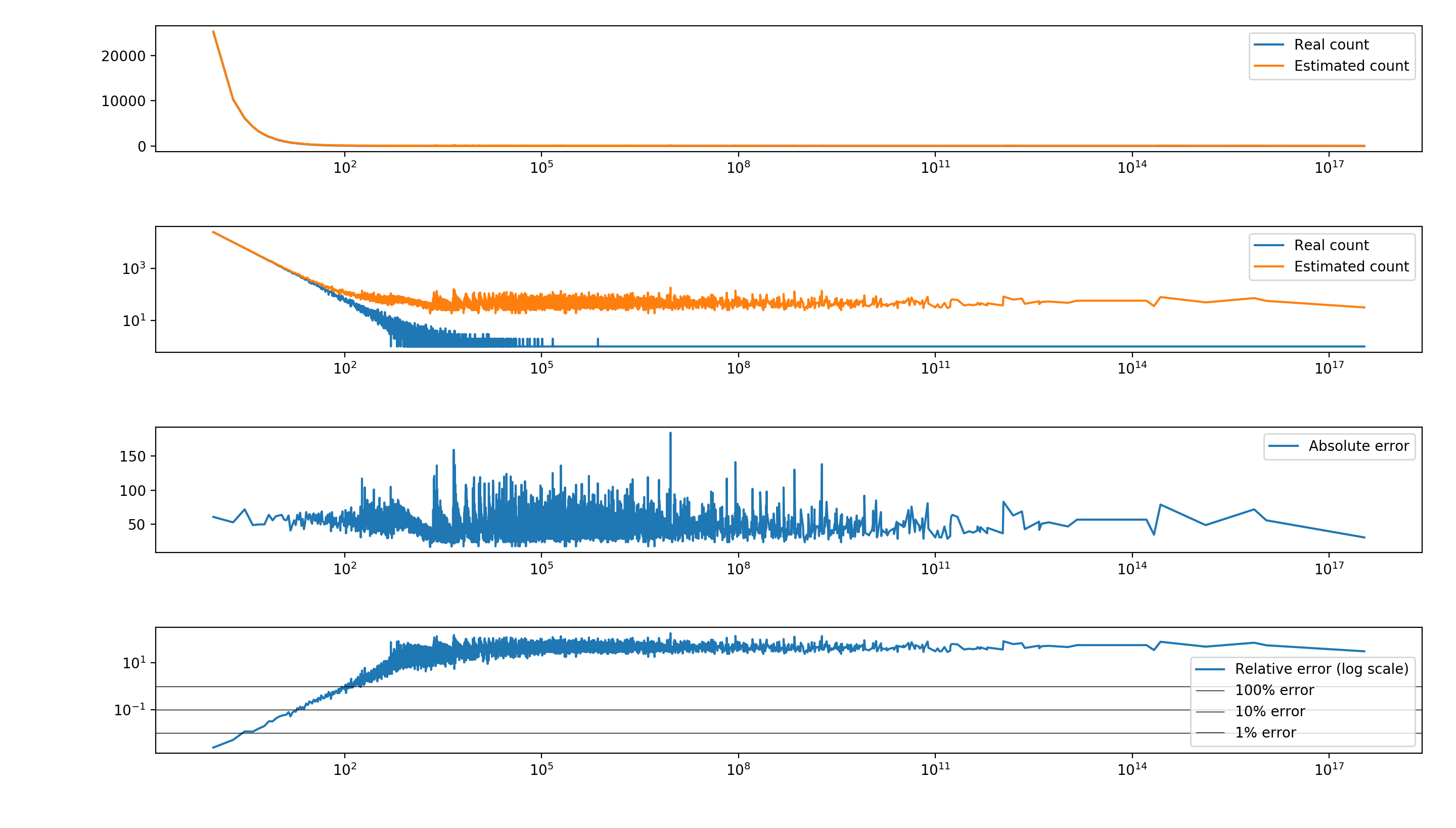
Some corrections for this behavior exist (for instance, subtracting the mean or the median of each row to “de-bias” the estimates), and are easy to implement. (See the full code here. The results are not strictly better, but can be preferred depending on your use case.
Bloom Filter
The Bloom filter is a probabilistic structure introduced in [4], used to test if a value belongs to a set or not. The test is guaranteed to be positive if the value has been seen, but it can return false positives with some probability.
The Bloom filter is extremely simple: it consists of an array \(A\) of \(M\) bits and a set of \(d\) independent hash functions. When a value \(v\) needs to be added, all bits corresponding to \(h_i(v)\) are flipped to 1. To check if a value was already encountered, it’s enough to verify if \(A_{h_i(v)} = 1\) for all \(i \in [0,d]\). The probability of returing a false positive clearly depends on \(M\), \(d\), and the number \(N\) of elements added to the set, and it can be shown to be around \(1 - e^{-dN/M}\). Viceversa, given \(N\) and a desired false positive rate, you can easily compute the optimal size of your structure, as: \(M = \lceil - N\log_2(p) / \ln(2) \rceil,~d = \lceil -\log_2(p) \rceil\)
Here’s a minimal python implementation. A slight more complete one is here.
import numpy as np

class BloomFilter:

    def __init__(self, M: int, d: int):
        self.M, self.d = M, d
        self.X = np.zeros(self.M, dtype=bool)
        self.hash = Hash(self.d, self.M)

    def add(self, x: int):
        self.X[self.hash(x)] = 1

    def __contains__(self, x: int):
        return np.all(self.X[self.hash(x)])
Below, the results of a quick example:
##### Bloom filter:
Num inserted values: 50000, min: 37, max: 999996
Desired FP rate: 5.00%, optimal size of Bloom filter: 311762 bits (with 5 hash functions)
Estimated FP rate: 4.76%
Desired FP rate: 10.00%, optimal size of Bloom filter: 239627 bits (with 4 hash functions)
Estimated FP rate: 9.55%
Desired FP rate: 20.00%, optimal size of Bloom filter: 167492 bits (with 3 hash functions)
Estimated FP rate: 19.92%
You can see here that, in order to have a 5% error rate for 50k distinct values, you needed to use 300k bits, which is obviously good if your items are so many and so complex that storing \(M\) bits rather then the items themselves is a big saving.
- G. Cormode, S. Muthukrishnan. An Improved Data Stream Summary: The Count-Min Sketch and its Applications.
- G. Cormode, S. Muthukrishnan. Approximating Data with the Count-Min Data Structure
- F. Deng, D. Rafiei. New Estimation Algorithms for Streaming Data: Count-min Can Do More
- H. Bloom. Space/Time Trade-offs in Hash Coding with Allowable Errors