On encoding angles for learning
Learning to predict angular (or circular/modular) quantities sounds like a pretty common task, and I happened to bump into similar issues a few times in the last couple of years. This had me wondering whether a small toy experiment could say something about the best way to encode angles in order to facilitate learning.
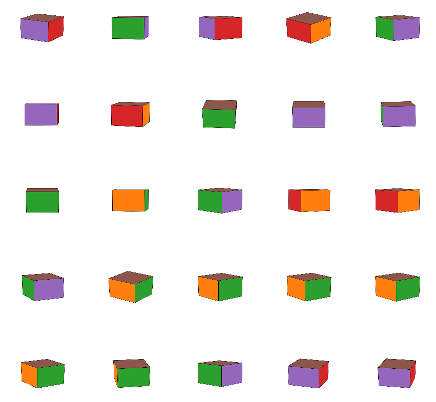
The idea is to generate an infinite sequence of images displaying a colored cube, with a randomly rotated point of view. Each side has a different color, so the network should learn extremely quickly to infer the view angle. To make things simpler, the network only needs to learn the azimuth angle, so the cubes are rotated around the z-axis. I’m also slightly changing the elevation angle in each image, to give a whiff of random “data augmentation”.
The code uses tensorflow 2.0 and was run (with minor modifications) in a Google colab. It’s all included in the hidden sections (click to expand).
(Code imports)
import random
import math
import numpy as np
from matplotlib import pyplot as plt
from scipy.spatial.transform import Rotation as R

import tensorflow as tf
from tensorflow.keras import layers as L
from tensorflow.keras.models import Model
from tensorflow.keras.utils import Sequence
Generating data
The images are generated on the fly with matplotlib. The function generate_random_image
generates an image (with random elevation angle in $[0,30]$) and returns the azimuth angle.
Here’s an example of images returned by the function (don’t mind the aliasing):
Code for image generation
from mpl_toolkits.mplot3d import Axes3D
import numpy as np
import matplotlib.pyplot as plt
from mpl_toolkits.mplot3d.art3d import Poly3DCollection

def cuboid_data(o, size=1):
    X = [[[0, 1, 0], [0, 0, 0], [1, 0, 0], [1, 1, 0]],
         [[0, 0, 0], [0, 0, 1], [1, 0, 1], [1, 0, 0]],
         [[1, 0, 1], [1, 0, 0], [1, 1, 0], [1, 1, 1]],
         [[0, 0, 1], [0, 0, 0], [0, 1, 0], [0, 1, 1]],
         [[0, 1, 0], [0, 1, 1], [1, 1, 1], [1, 1, 0]],
         [[0, 1, 1], [0, 0, 1], [1, 0, 1], [1, 1, 1]]]
    X = np.array(X).astype(float)
    X -= 1/2 #move the center of the cube in the origin
    X *= size
    X += np.array(o)
    return X

def plot_cube(rotation=None):
    colors = [f"C{i}" for i in range(6)]
    size = 1
    position = [0, 0, 0]
    cube = cuboid_data(position, size=size)
    if rotation is not None:
        cube = cube @ rotation.T
    return Poly3DCollection(cube, facecolors=colors, edgecolor="k")

def generate_random_image(rotate_elevation=False):
    """
    Generate image of a cube with a random rotation
    """
    plt.ioff() #to disable "inline mode" that automatically displays figures in a notebook

    fig = plt.figure()
    ax = fig.gca(projection='3d')#, proj_type = 'ortho') #ortho if want to remove perspective effects
    pc = plot_cube()
    ax.add_collection3d(pc)
    ax.set_xlim([-.5,.5])
    ax.set_ylim([-.5,.5])
    ax.set_zlim([-.5,.5])
    ax.set_axis_off()

    azim_rot = random.random()*360
    if rotate_elevation:
        elev_range = 30
        elev = random.random()*elev_range
    else:
        elev = 10
    ax.view_init(elev=elev, azim=azim_rot)

    fig.canvas.draw()
    fig.tight_layout(pad=0)
    data = np.frombuffer(fig.canvas.tostring_rgb(), dtype=np.uint8)
    data = data.reshape(fig.canvas.get_width_height()[::-1] + (3,))
    plt.close()

    return data, azim_rot
%matplotlib inline

fig, axes = plt.subplots(5,5, figsize=(15, 15))

for ax in axes.ravel():
    data, y = generate_random_image(rotate_elevation=True)
    ax.imshow(data)
    ax.axis('off')
plt.show()
Encoding & learning angles
The main issue of learning angular quantities is, of course, the fact that $\alpha = \alpha + 2k\pi$ for any $k \in \mathbb{N}$. In practical terms, this means that our model will need to understand that 0 and 358 are closer than, say, 50 and 85.
What I’m trying here are the following simple approaches1:
- raw angle $\alpha \in [0,360]$ – just like that. Yes, it’s not going to behave well.
- normalized angle $\alpha \in [0,1]$ – normalizing the inputs is always a good idea. Still this doesn’t solve the crux of the issue.
- encoding the angle on the unit circle as $(cos(\alpha), sin(\alpha))$ – this avoids altogether the discontinuity, moving to a 2d plane.
- binning – this sounds like a very sensible way to go. After all, nn are great at multi-category classification, even with a high number of classes. Classes are not ordered, which is a downside but also a plus, meaning that we don’t need to worry about the discontinuity around 360.
The different approaches can be easily incapsulated in an infinite keras Sequence,
that needs to be initialized with the type of desired encoding, and will return
the image + the corresponding label.
Code for the Keras data generator
def encode_angle(angle, kind='raw_angle'):
    if kind == 'raw_angle':
        return angle
    if kind == 'scaled_angle':
        return angle/360
    if kind == 'cossin':
        return [math.cos(angle/360*2*math.pi), math.sin(angle/360*2*math.pi)]
    if kind.startswith('binned_'):
        num_bins = int(kind.split("_")[1])
        idx = int(angle / 360 * num_bins) % num_bins
        one_hot = np.zeros(num_bins)
        one_hot[idx] = 1
        return one_hot

def decode_angle(y, kind='raw_angle'):
    if kind == 'raw_angle':
        return y
    if kind == 'scaled_angle':
        return y * 360
    if kind == 'cossin':
        c, s = y
        return math.atan2(s, c)*180/math.pi
    if kind.startswith('binned_') or kind.startswith('softbinned_'):
        num_bins = int(kind.split("_")[1])
        delta = 360 / num_bins
        idx = np.argmax(y)
        return float((idx + .5) * delta) #for decoding, get middle of the bin.

class RandomlyRotatedCube(Sequence):

    def __init__(self, batch_size, kind, num_batches=10):
        self.batch_size = batch_size
        self.kind = kind
        self.num_batches = num_batches

    def __len__(self):
        return self.num_batches #arbitrary number of batches in an epoch

    def __getitem__(self, idx): #get idx-th batch
        X, Y = [], []
        for i in range(self.batch_size):
            data, angle = generate_random_image(rotate_elevation=True)
            y = encode_angle(angle, self.kind)
            X.append(data)
            Y.append(y)
        return np.array(X).astype(float)/255, np.array(Y).astype(float)
The model used for the task has a CNN backbone, with a head classifier that needs to be slightly adapted for each encoding method:
- raw angle: just a linear activation, and mean squared error as a loss; this of course is bad since it misses completely the fact that +180 and -180 or 0 and 360 are exactly the same angle.
- scaled angle: using a sigmoid activation and a binary crossentropy loss. It should be a bit better behaved but has the same issue of 1).
- (cos,sin) encoding: $tanh$ activation to enforce outputs to be in $(-1, +1)$, and mse loss
- bins: softmax activation with categorical crossentropy.
def build_model(kind, **kwarg):
    input = L.Input(shape=(288, 432, 3))
    x = L.Conv2D(8, 5, activation='relu')(input)
    x = L.MaxPool2D(5)(x)
    x = L.Conv2D(16, 3, activation='relu')(x)
    x = L.MaxPool2D(3)(x)
    x = L.Conv2D(32, 3, activation='relu')(x)
    x = L.Flatten()(x)
    x = L.Dense(50, activation='relu')(x)

    if kind == 'raw_angle':
        output = L.Dense(1, activation='linear')(x)
        model = Model(input, output)
        model.compile(optimizer='adam', loss='mse')
    if kind == 'scaled_angle':
        output = L.Dense(1, activation='sigmoid')(x)
        model = Model(input, output)
        model.compile(optimizer='adam', loss='binary_crossentropy')
    if kind == 'cossin':
        output = L.Dense(2, activation='tanh')(x)
        model = Model(input, output)
        model.compile(optimizer='adam', loss='mse')
    if kind.startswith('binned_'):
        num_bins = int(kind.split("_")[1])
        output = L.Dense(num_bins, activation='softmax')(x)
        model = Model(input, output)
        model.compile(optimizer='adam', loss='categorical_crossentropy', metrics=['accuracy'])
    return model
Code for training
KINDS = ['raw_angle', 'scaled_angle', 'cossin', 'binned_4', 'binned_8', 'binned_32', 'binned_360']
NUM_EPOCHS = 10
trained_models = {}
test_results = {}
for kind in KINDS:
    print(kind)
    try:
        model = tf.keras.models.load_model(f'model_{kind}.h5')
        print(f"Loaded {kind} model from disk")
    except Exception as e:
        print("Training:", e)
        model = build_model(kind)
        train_generator = RandomlyRotatedCube(16, kind, 20)
        model.fit_generator(train_generator, epochs=NUM_EPOCHS, shuffle=False)
        model.save(f'model_{kind}.h5')
    test_res = test_model(model, kind=kind, N=100)
    print(f"{kind} test result: {test_res}")
    trained_models[kind] = model
    test_results[kind] = test_res
For these experiments, I’m using the 4 approaches described above, using 8, 32, and 360 bins. The training takes ~10s per epoch (each epoch has 20 batches x 16 examples) on Colab’s NVidia P100. I let them run for 10 epochs. The loss gets very small in all cases; the task is indeed easy.
Let’s see how the models compare on “unseen” data. [This is not completely fair; given the way in which the training images are generated, one can expect that most (all?) examples seen in test will be almost identical to something already seen in training.]
I generated 200 samples and computed the mse (adjusted for angles) and an accuracy with several error tolerances: 1°, 5°, 10°, and 25°.
Code for testing
%matplotlib inline
def angle_abs_dist(alpha, beta):
    return min(abs(alpha-beta), abs(alpha-beta-360))

def test_model(model, *, kind='raw_angle', seed=55, N=100, verbose=False, resolutions=[1,5,10,25], return_output=False):
    mse = 0.0
    errors = {r:0 for r in resolutions}
    random.seed(seed)
    outputs = np.zeros((N,2))
    for i in range(N):
        data, angle = generate_random_image()

        y_hat = model(data[None].astype(np.float32)/255).numpy().squeeze()
        angle_hat = decode_angle(y_hat, kind=kind)

        outputs[i,:] = (angle, angle_hat)

        dist = angle_abs_dist(angle, angle_hat)
        mse += dist**2

        if verbose:
            print(f"y_hat={y_hat}, angle={angle}, angle_hat={angle_hat}, dist={dist}")

        for r in resolutions:
            if dist > r:
                errors[r] += 1

    mse /= N
    acc = {r: (N - errors[r])/N for r in resolutions}
    if return_output:
        return {"mse": mse, "acc": acc, "output": outputs}
    else:
        return {"mse": mse, "acc": acc}

test_results = {kind: test_model(trained_models[kind], kind=kind, N=200, verbose=False, return_output=True) for kind in KINDS}

fig, ax = plt.subplots(len(test_results),1,sharex=True, figsize=(10,10))
for i, (k,r) in enumerate(test_results.items()):
    print(i, k, r["mse"], r["acc"])
    ax[i].plot(sorted((x,y) for (x,y) in r["output"]), label=k)
    ax[i].legend()
plt.show()
| Encoding | MSE | acc @1° | acc @5° | acc @10° | acc @25° |
|---|---|---|---|---|---|
| raw_angle | 1057.69 | 0.055 | 0.205 | 0.34 | 0.73 |
| scaled_angle | 171.53 | 0.045 | 0.305 | 0.65 | 0.97 |
| cossin | 6.53 | 0.32 | 0.92 | 1.0 | 1.0 |
| binned_4 | 724.84 | 0.015 | 0.08 | 0.185 | 0.51 |
| binned_8 | 1268.3 | 0.04 | 0.28 | 0.475 | 0.98 |
| binned_32 | 11.44 | 0.19 | 0.865 | 1.0 | 1.0 |
| binned_360 | 6654.73 | 0.185 | 0.575 | 0.72 | 0.84 |
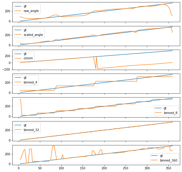
Loking at the results, it appears that encoding angles as $(cos, sin)$ makes sense, and it’s comparable to using a 32-bins approach.
Using 360 bins yields a slower convergence, while the results show that regressing the angles should generally be avoided (though scaling between 0 and 1 is beneficial).
A plus of the binned approach is that one could use a kind of “multiple resolution” loss, where the loss is obtained summing the errors at different binning resolutions. This might help speeding up convergence while reaching finer-grained results.
Plotting the ground truth vs the predictions, it’s easy to see how the discontinuity at 360 significantly affects the regression approach, while the binned and the cossin approaches are essentially immune to it.
-
Of course there must be plenty of literature dealing with the subject, but I admit I didn’t take a serious look at previous work. My guess is most ideas I’m trying here are folklore. ↩