Plotting mathematical functions in... BASIC
For most people nowadays the first programming language is python or javascript. Once upon a time that was not the case, and probably BASIC was the one where most millennials got their feet wet.
That actually never happened for me – I barely knew what “programming” meant before my first university courses, which technically makes Assembly and C my first programming languages. Last week I was skimming through an undergrad level Calculus book (old, but still used by students in Italy), and there I found a juicy chapter on plotting mathematical functions (with 1 or 2 variables) with.. BASIC.
I was rather intrigued by the nice looking plots, and how the code actually looked pretty terse! I had to try and replicate those results.
BASIC is more a family of languages than a single one. I picked one that I could
easily install on ubuntu (sudo apt install yabasic) and was good to go.
This turned out to be a slightly more modern dialect than the one in the book, but the gist is the same.
2d plots
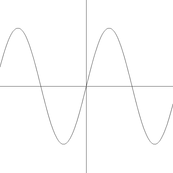
First thing: plotting single-variable functions.
W = 600
H = 600
OPEN WINDOW W,H

X0 = W/2
Y0 = H/2
LINE 0,Y0,W,Y0 //X-AXIS
LINE X0,0,X0,H //Y-AXIS

SUB FUN(X)
    RETURN 200*SIN((X/50))
END SUB

FOR X = 0 TO W
    Y = -FUN(X - X0) + Y0 //invert y coordinate and center in Y0
    LINE X,Y
NEXT X
In the first block I’m opening a new window with size (W,H).
Then I’m plotting the x and y axis in the middle of the window.
FUN is the function I want to plot. Finally, a for loop where I need to convert the y
value in the actual “window” coordinate (in the output window, the point (0,0) is the upper left corner).
The LINE X,Y instruction does the heavy lifting here: if no LINE was previously called, the current point is set to X,Y;
otherwise, it draws a line from the previous point to X,Y. Pretty nifty and concise.
This is the glorious result:
Note that, in the function definition, one needs to make sure the plot can actually be visualized in the window in a decent way – meaning, we need to scale and/or translate it so the window contains something meaningful.
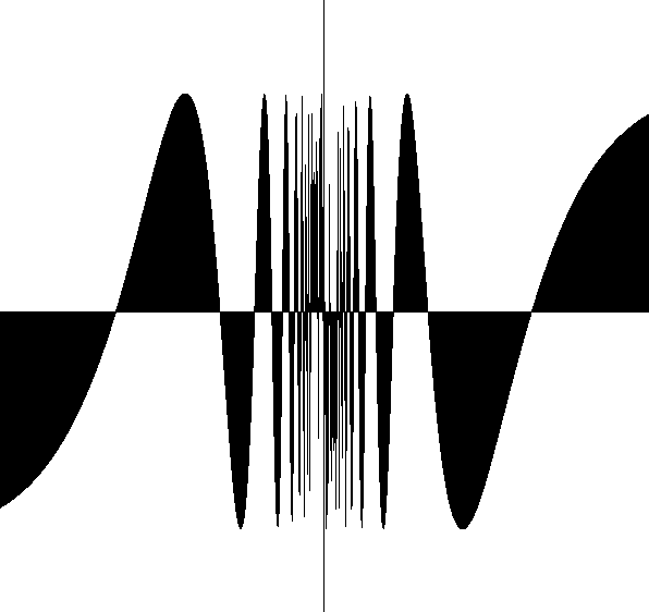
Another easy trick shown in the book is how we can plot a filled curve, where for each X we draw a line between (X,Y) and the x-axis:
FOR X = 0 TO W
    Y = -FUN(X - X0) + Y0 //invert y coordinate and center in Y0
    LINE X,Y0,X,Y
NEXT X
With $y = sin(1/x)$ (and some appropriate scaling) this is what you get:
3d plots
Plotting 2-variables functions in a 3d space is a bit trickier.
Given $Z=F(X,Y)$, one needs to transform the $(X,Y,Z)$ point into $(U,V)$-coordinates, that is, the coordinates relative to the window.
Let’s assume that $X$ is the axis which is normal to the screen, while $Z$ is the vertical axis and $Y$ the lateral axis.
The idea is to draw lines (“slices” of the surface) connecting consecutive points with constant $X$. To give depth and
obtain a 3d-ish view, each line is shifted up and right by a small amount of pixels (SHIFT).
W = 1400
H = 1000
OPEN WINDOW W,H
U0 = W/2
V0 = H/2

SUB FUN(X,Y)
    //Define function here
END SUB

SHIFT = 4
X = 0
NUM_LINES = 80
RADIUS = 600
FOR I=-NUM_LINES/2 TO NUM_LINES //number of lines to plot
    X = I*(W/NUM_LINES)
    NEW CURVE
    FOR Y=-W TO W
        Z = FUN(X,Y)
        U = Y + U0 + I*SHIFT
        V = -Z + V0 - I*SHIFT
        LINE U,V
    NEXT Y
NEXT I
With the NEW CURVE instruction, we stop keeping track of the latest point and a new LINE is started.
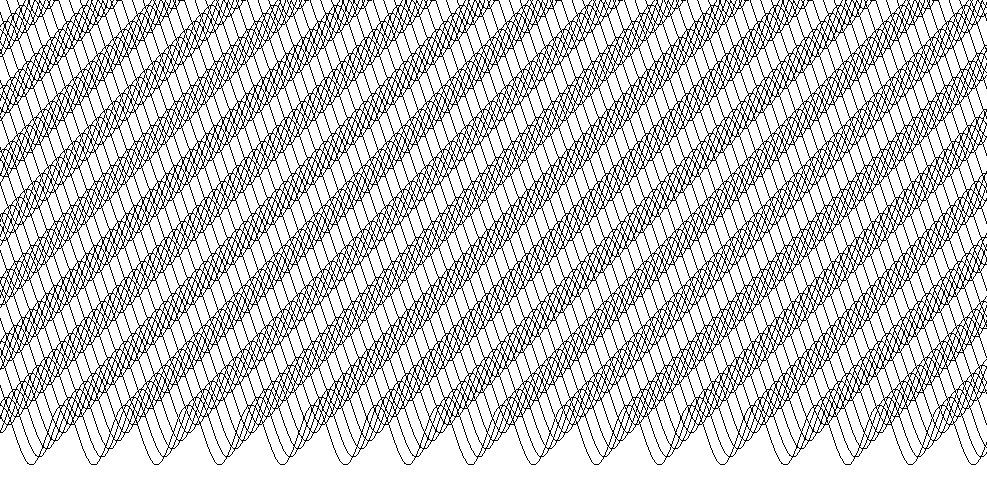
This code returns a 3d plot, but the result is a bit of a mess even for a simple function like $z = sin(y)$:
To avoid this issue, one needs to avoid printing lines that are covered by surfaces that are in front of them. We can do that storing the max and min $V$-value for each $U$, so that one can check if a point should be visible.
DIM MAX_V(W), MIN_V(W)
FOR I=0 to W
    MAX_V(I) = -10000000
    MIN_V(I) = 10000000
NEXT I

SHIFT = 4
X = 0
NUM_LINES = 80
RADIUS = 600
FOR I=-NUM_LINES/2 TO NUM_LINES //number of lines to plot
    X = I*(W/NUM_LINES)
    NEW CURVE
    FOR Y=-W TO W
        Z = FUN(X,Y)
        U = Y + U0 + I*SHIFT
        V = -Z + V0 - I*SHIFT
        IF U >= 0 AND U < W AND V < MAX_V(U) AND V > MIN_V(U) THEN
            NEW CURVE
            CONTINUE
        ENDIF
        IF U >= 0 AND U < W AND V > MAX_V(U)
            MAX_V(U) = V
        IF U >= 0 AND U < W AND V < MIN_V(U)
            MIN_V(U) = V
        LINE U,V
    NEXT Y
NEXT I
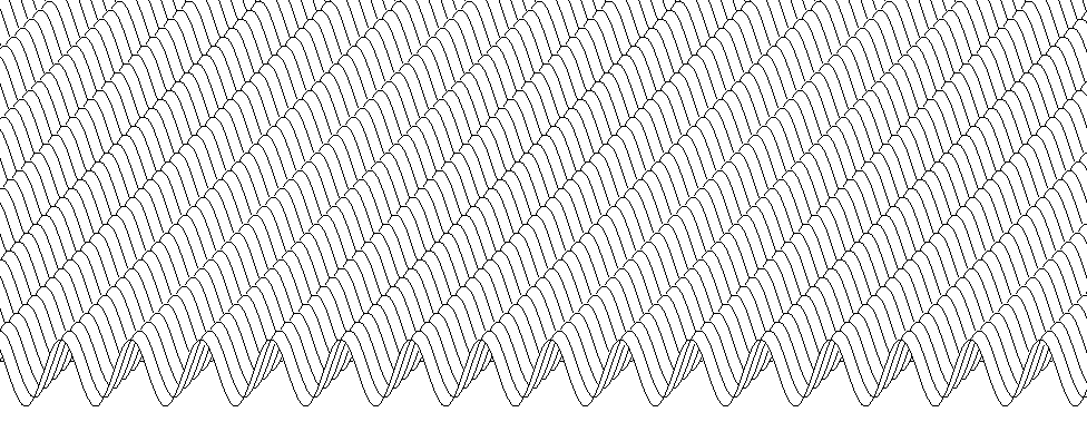
This is the correct result for $z = sin(y)$:
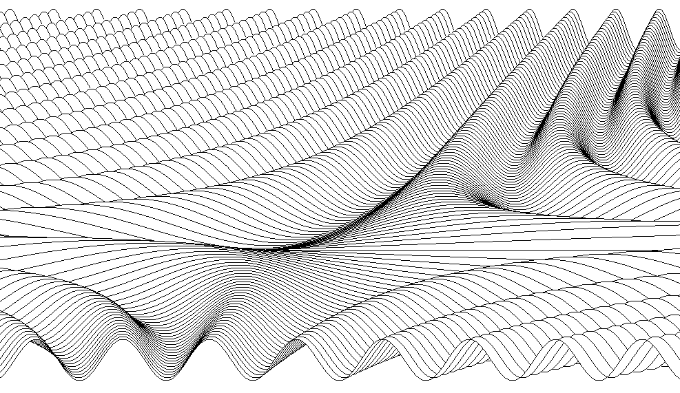
And here’s another example with $z = sin(xy)$:
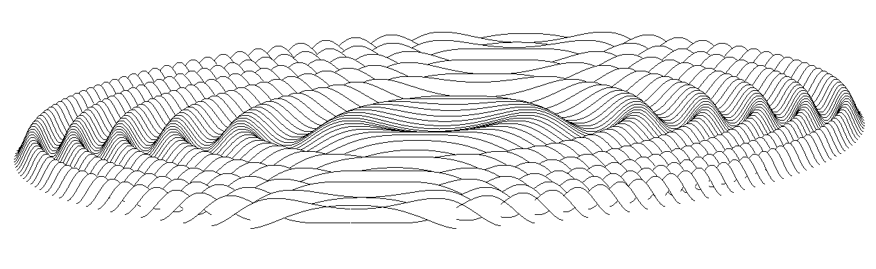
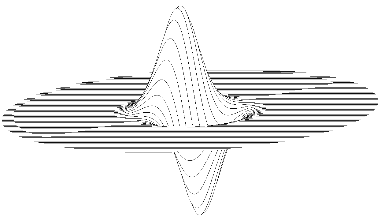
We can also add some other eye-candy, like limiting the (X,Y) domain to a circle. Here $sin(x^2 + y^2)$ and $(x-y)e^{-(x^2 + y^2)}$: