Procedural generation of images with.. integer programming?
In computing, procedural generation is a method of creating data algorithmically as opposed to manually, typically through a combination of human-generated assets and algorithms coupled with computer-generated randomness and processing power.
Procedural generation is common in computer graphics and game design to generate textures, terrain, or even for level/map design. Generative art is also all the rage now, thanks to all the NFT hype (I won’t comment further here..).
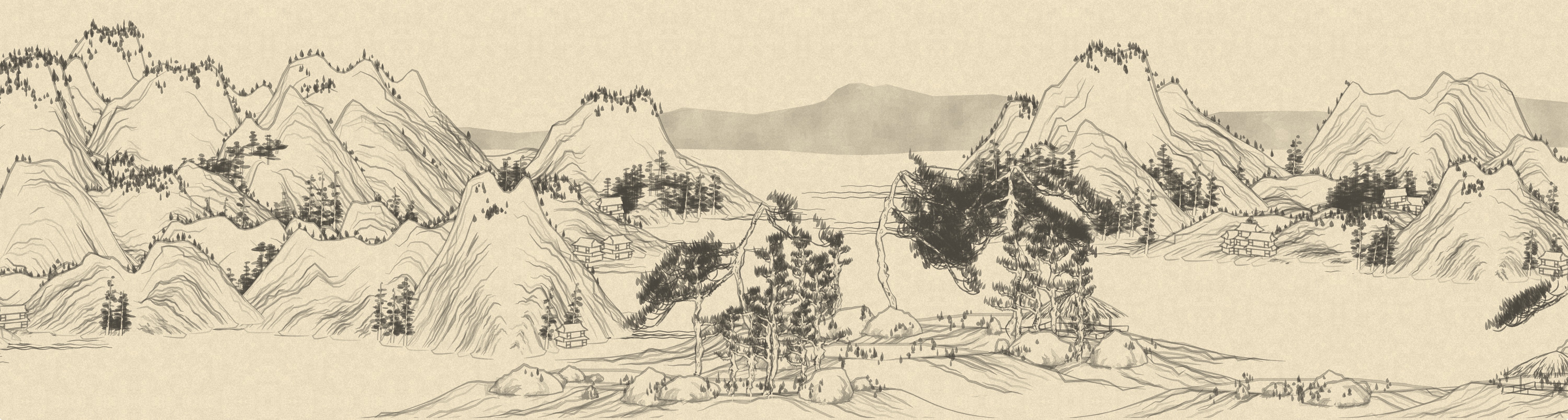
There are so many methods for procedural generations, and so many people that do great stuff online. As an example, a few days ago I stumbled upon this delightful infinitely-scrolling Chinese landscape generator (here):
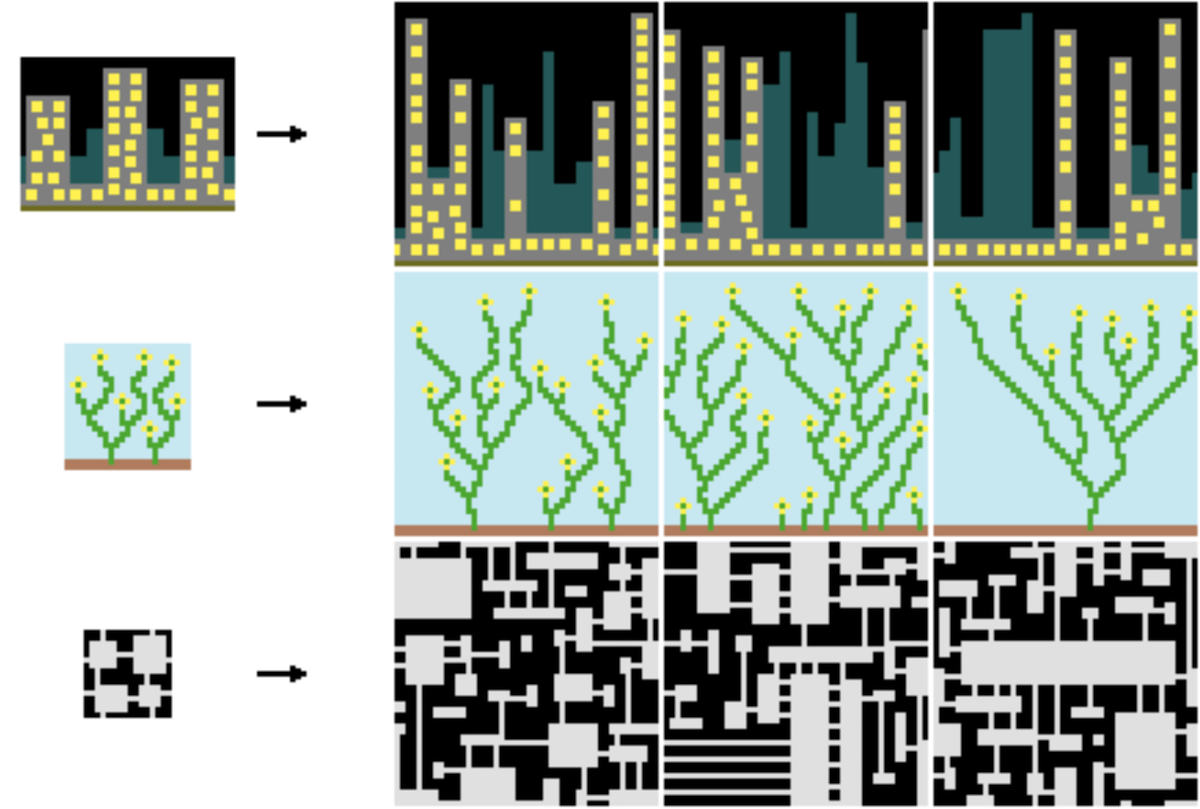
While this Chinese landscape is generated using an ad-hoc algorithm, there are several popular and more general techniques used in the procedural generation community, such as the so-called Wave Function Collapse algorithm by Ex-Utumno. WFC generates images that are locally similar to an input bitmap. The algorithm splits the input image into small tiles (say, 2x2), and tries to infer simple constraints for each unique tile (for example, a tile with a road exiting on the right can only be adjacent to a tile with a road entering from the left). Then, it builds a new image generating tiles (with randomness) and propagating constraints so that we find a feasible solution with high probability.
I wanted to try something like that myself, but, being extremely lazy, I didn’t feel like implementing a constraint propagation algorithm from scratch (though that sounds fun!).
So I decided to try an extremely dumb technique, but that required almost 0 effort on my part: why not formulating the problem as an Integer Program?
Let’s define the output image as a graph (V,E) where each node is a tile and the arcs link to the adjacent tiles.
Say we have 4 tile patterns: T = {sea, coast, land, mountain}. We set a desired output distribution (say, 40% of the cells must be sea, 20% must be land, etc..).
Then it’s enough to formulate a model as:
where $x_{vt}$ is 1 if the pattern $t$ is assigned to the cell $v$, and we minimize the distance from the desired distribution. (The absolute value in the objective function can be easily removed adding a few auxiliary variables and constraints).
If there are two patterns $(t_1,t_2)$ that can’t be adjacent, such as sea and mountain, we add:
\[\begin{align} & x_{ut_1} + x_{vt_2} \leq 1 \qquad&\forall (u,v) \in E\\ \end{align}\]And if we want a pattern $t_1$ to have at least an adjacent cell with pattern $t_2$ (say, coast must be next to sea):
\[\begin{align} & \sum_{u \in adj(v)} x_{ut_2} \geq x_{vt_1} \qquad&\forall v \in V\\ \end{align}\](Here's the Julia code to define and solve the model with JuMP and SCIP.)
I = 1:I
J = 1:J
V = [(i,j) for i in I for j in J]

adj = (i,j) -> [tuple(([i,j] + k)...) for k in [[-1,0],[+1,0],[0,-1],[0,1]] if all([i,j] + k .∈ (I,J))]

E = [(u,tuple(v...)) for u in V for v in adj(u...)]
T = [:land, :sea, :coast, :mountain];
N = length(V)
Desired = Dict(:land => round(0.4*N), :sea => round(0.4*N), :coast => round(0.1*N)) #mountain: what's left
Desired[:mountain] = N - sum(values(Desired))

model = Model(SCIP.Optimizer);

@variable(model, x[V,T], Bin);
@variable(model, η[T] >= 0)

@constraint(model, assignment[v in V], sum(x[v,t] for t in T) == 1);

@constraint(model, sealand[(u,v) in E], x[u,:land] + x[v,:sea] <= 1);
@constraint(model, seamountain[(u,v) in E], x[u,:mountain] + x[v,:sea] <= 1);
@constraint(model, coastmountain[(u,v) in E], x[u,:mountain] + x[v,:coast] <= 1);

@constraint(model, landcoast[v in V], sum(x[u,:land] for u in adj(v...)) >= x[v,:coast]);
@constraint(model, seacoast[v in V], sum(x[u,:sea] for u in adj(v...)) >= x[v,:coast]);
@constraint(model, mountainchain[v in V], sum(x[u,:mountain] for u in adj(v...)) >= x[v,:mountain]);

@constraint(model, major1[t in T], η[t] >= sum(x[v,t] for v in V) - Desired[t]);
@constraint(model, major2[t in T], η[t] >= - sum(x[v,t] for v in V) + Desired[t]);

@objective(model, Min, sum(η[t] for t in T));

Random.seed!(42)
# Fix randomly 3 cells
for t in T
    v = Random.rand(V)
    println("Fixing $v to $t")
    fix(x[Random.rand(V),t], 1.0, force=true)
end

optimize!(model)
println("Optimal value: ", objective_value(model))

xval = value.(x) .> 1 - 1e-5 #circa 1

Color = Dict(:land => :green, :sea => :blue, :coast => :yellow, :mountain => :light_black);
for i in I
    for j in J
        for t in T
            if x[(i,j),t]
                printstyled(" ",  color=Color[t], reverse=true)
            end
        end
    end
    print("\n")
end
Solving to optimality for large-ish images is super slow - my model is as naive as it gets, and finding an optimal solution is really pointless, we’d rather generate quickly multiple feasible solutions. Here’s a result for the simple example in the code above:
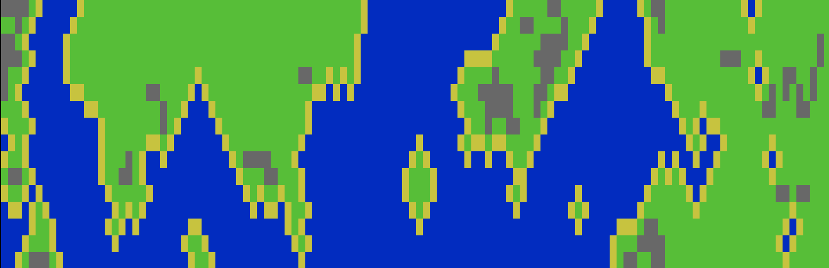
Not too bad: it does look like a big map with recognizable features such as lakes, mountain chains, islands. This is not a recommended approach, it’s very dumb – still, I suspect that with some tuning and clever modeling tricks one could 1) generate very interesting/complex patterns 2) greatly reduce the solving time. After all, somebody already thought of ways to generate art with mathematical optimization and even wrote a book about it.